CAC vs LTV Data Model: Optimize Unit Economics with SQL
Calculating Customer Acquisition Cost (CAC) vs. LTV: The Ultimate Data Model
The calculation of Customer Acquisition Cost (CAC) and Lifetime Value (LTV) forms the definitive bedrock of modern unit economics, dictating capital allocation, growth velocity, and ultimate enterprise valuation across both software-as-a-service (SaaS) and e-commerce business models. Historically, organizations relied on static spreadsheets, blended averages, and generalized assumptions to calculate these figures, often masking profound operational inefficiencies. As macroeconomic conditions have shifted away from growth-at-all-costs toward sustainable profitability and efficient cash flow management, the demand for absolute precision in unit economics has escalated.
The proliferation of digital touchpoints, the transition toward product-led growth (PLG) and usage-based pricing, and the increasing complexity of omnichannel marketing have rendered traditional, static financial models entirely obsolete. To accurately measure the efficiency of go-to-market (GTM) motions, modern data teams must architect dynamic, code-driven data models within cloud data warehouses utilizing transformation frameworks like dbt (data build tool) and automated ingestion pipelines. This exhaustive analysis deconstructs the mathematical definitions, architectural requirements, dimensional modeling paradigms, and structured query language (SQL) implementations necessary to build the definitive data model for CAC, LTV, marketing attribution, and revenue retention.

The Mathematical and Strategic Foundations of Unit Economics
Before architecting the underlying data warehouse schema, the mathematical and operational definitions of the financial metrics must be rigidly established. Discrepancies in how disparate departments calculate these numbers frequently lead to distorted LTV:CAC ratios, creating a false sense of security while simultaneously draining cash reserves.

Deconstructing Customer Acquisition Cost (CAC)
Customer Acquisition Cost represents the total financial investment required to convert a prospective buyer into a paying customer. While the basic arithmetic appears straightforward, the complexity lies in accurately defining the cost numerator and correctly attributing the customer denominator over the appropriate temporal horizon. Data architecture must differentiate between distinct classifications of CAC to provide actionable visibility across the executive suite and marketing operations.
| CAC Classification | Mathematical Definition | Strategic Application and Limitations |
|---|---|---|
| Blended CAC | Total sales and marketing expenditures divided by all new customers acquired, regardless of source. | Provides a high-level macroeconomic pulse of the business. Useful for board reporting but dangerous for channel optimization, as high-volume organic growth obscures the inefficiencies of paid channels. |
| Paid CAC | Direct advertising and media spend divided strictly by the volume of customers acquired through paid channels. | Isolates the performance of performance marketing capital. Essential for media buying, budget allocation, and ROAS (Return on Ad Spend) optimization, yet ignores the human capital required to run the campaigns. |
| Fully Loaded CAC | Includes direct ad spend, all marketing and sales salaries, commissions, agency fees, software tooling, and allocated overhead divided by new customers. | The most accurate reflection of true enterprise profitability. Failing to include salaries and software overhead can artificially understate acquisition costs by factors of two to three. |
The mathematical formulation for Fully Loaded CAC is expressed as:
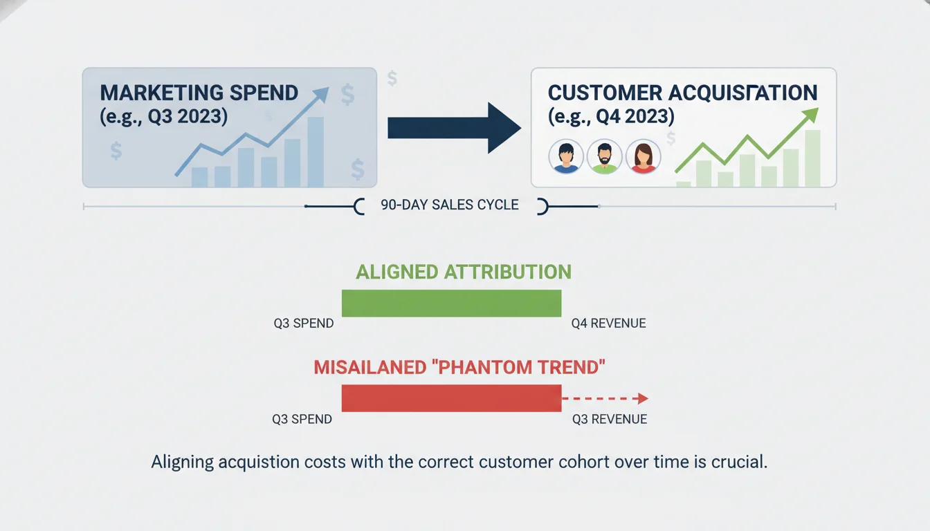
A critical failure point in legacy financial modeling is the misalignment of time horizons. If a business-to-business (B2B) enterprise operates with a 90-day sales cycle, dividing October’s marketing spend by October’s new customers produces a phantom trend. The customers who closed in October were likely generated by marketing capital deployed in July or August. A robust data model must apply lagged cohort attribution, aligning the cohort of acquired customers with the specific capital deployed during their actual acquisition cycle to prevent severe analytical distortion.
Deconstructing Customer Lifetime Value (LTV)
Lifetime Value models the total economic benefit a business expects to realize from a customer over the entire duration of their commercial relationship. The architectural requirements for calculating LTV differ fundamentally depending on the underlying business model and whether the analytical approach is historical or predictive.
In a software-as-a-service (SaaS) or subscription model, revenue is recognized on a recurring schedule, rendering the churn rate the primary determinant of customer lifespan. The standard SaaS LTV formula assumes an infinite geometric series based on recurring revenue and margin:
In contrast, e-commerce data models must account for discrete, non-contractual transactions. Because there is no explicit cancellation event in retail, the focus shifts away from explicit churn toward purchase frequency, average order value (AOV), and predictive lifespan modeling:
A pervasive data modeling error across both sectors is utilizing top-line revenue rather than gross profit. If a direct-to-consumer (DTC) apparel brand has an LTV of $500 based on top-line revenue but operates on a 40% gross margin due to the high cost of goods sold (COGS) and fulfillment, the true economic value delivered to the business is only $200. Failing to apply the margin adjustment leads to artificially inflated LTV:CAC ratios. For example, if the acquisition cost is $150, a revenue-based LTV ratio appears healthy at 3.3:1, but the accurate profit-based ratio is a dismal 1.3:1, indicating a business model that is barely breaking even and rapidly burning cash.
The Evolution from Static Ratios to Cohort Payback Periods
The traditional industry benchmark dictates that a healthy enterprise should maintain an LTV:CAC ratio of 3:1 or higher, signifying that the lifetime gross profit is three times the cost of acquisition. Ratios closer to 1:1 indicate value destruction, while ratios exceeding 5:1 suggest the organization is underinvesting in growth and leaving market share to competitors.
However, the rapid expansion of bottom-up software sales, product-led growth (PLG) motions, and usage-based pricing models has exposed the fragility of static LTV assumptions. Static LTV calculations rely on the flawed premise of a constant churn rate and linear pricing. In modern environments, revenue fluctuates dynamically across the lifecycle through seat expansions, cross-sells, usage overages, and tier downgrades.
Consequently, advanced data teams are shifting their focus away from static LTV:CAC ratios toward Cohort Gross Margin Payback. The payback period calculates the exact duration required to recover the fully loaded customer acquisition cost.
A highly optimized data model tracks payback dynamically across temporal cohorts, targeting a recovery period of 5 to 12 months. This metric is significantly more resilient to the theoretical assumptions of lifetime value, grounding the analysis in actual cash flow dynamics and immediate capital efficiency.
Architectural Foundations of the Modern Data Stack
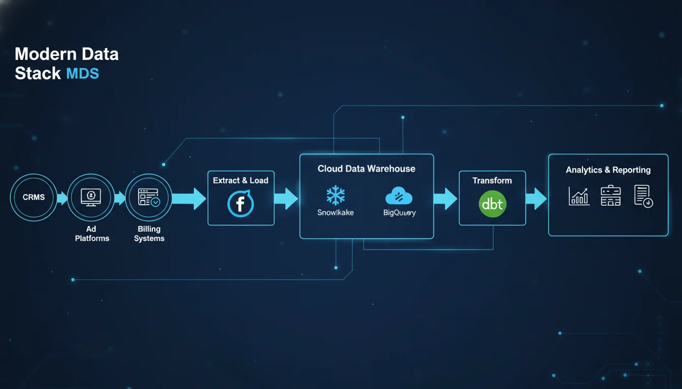
To calculate dynamic, cohort-based, fully loaded unit economics, data must be extracted from highly disparate source systems, ranging from customer relationship management (CRM) platforms and billing gateways to advertising networks and behavioral tracking pixels. The Modern Data Stack (MDS) has emerged as the definitive architecture for this unification process, typically comprising a dedicated extraction and loading tool, a highly scalable cloud data warehouse, and a robust transformation framework.
The Extract and Load (EL) Paradigm
The traditional Extract, Transform, Load (ETL) paradigm has been largely superseded by Extract, Load, Transform (ELT). Automated data movement platforms like Fivetran handle the computationally heavy and maintenance-intensive process of extracting data from complex application programming interfaces (APIs) such as Salesforce, Stripe, Google Ads, and Meta. These tools load the data securely into the warehouse in its raw, normalized state. Decoupling extraction from transformation ensures that raw historical data is persistently available for auditing, and it prevents upstream API schema changes from breaking downstream business logic.
Cloud Data Warehousing: Snowflake and BigQuery
The central nervous system of the ultimate data model is the cloud data warehouse. Snowflake and Google BigQuery dominate the enterprise landscape, though their underlying economic architectures require distinct data engineering strategies.
| Platform Architecture | Compute and Storage Model | Financial Operations (FinOps) Considerations |
|---|---|---|
| Snowflake | Separated storage and compute. Billing is driven by the active uptime of provisioned “Virtual Warehouses” (measured in credits). | Highly optimized for complex dimensional modeling and concurrency. Marketing teams can run heavy attribution queries on one warehouse while finance runs MRR aggregations on another, eliminating resource contention. |
| Google BigQuery | Serverless, on-demand execution. Billing is traditionally driven by the volume of data scanned per query (per terabyte). | Engineers must rigorously enforce table partitioning (e.g., by date) and clustering. Failing to partition large web event tables during multi-year cohort analyses will result in massive, unexpected scan costs. |
Data Transformation via dbt (data build tool)
Once the raw data resides within the warehouse, it must be cleansed, joined, and transformed into the analytical entities required for CAC and LTV calculations.
The data build tool (dbt) has established itself as the industry standard for this semantic layer, empowering analytics engineers to write modular, version-controlled SQL. The integration of these tools has become so foundational that Fivetran and dbt Labs announced a definitive merger agreement in October 2025, creating a unified platform for open data infrastructure that seamlessly bridges ingestion and transformation while maintaining open-source flexibility.
Within a sophisticated dbt project, transformations are structured across strict hierarchical layers to ensure data governance, reusability, and scalability:
- Staging Models (stg_): These serve as a one-to-one representation of raw source tables. This layer handles fundamental cleaning tasks: column renaming to enforce naming conventions, data type casting, timezone normalization (e.g., converting all timestamps to UTC), and basic JSON parsing. No complex joins or business logic are permitted at this stage.
- Intermediate Models (int_): The operational core of the pipeline. This layer joins data across disparate systems, resolves user identities, stitches anonymous web sessions, and calculates preliminary mathematical weights for attribution models.
- Mart Models (fct, dim): The final, production-grade tables exposed to Business Intelligence (BI) tools and downstream consumers. These are heavily denormalized fact and dimension tables optimized for instantaneous querying and reporting.
Dimensional Modeling for Go-To-Market Analytics
The ultimate data model relies on the Kimball dimensional modeling methodology, specifically leveraging the Star Schema architecture. This structural design denormalizes data by separating quantitative, highly granular event data into central Fact tables, surrounded by descriptive, categorical data housed in Dimension tables.
A properly designed Entity-Relationship Diagram (ERD) is critical to map this schema. A common, catastrophic error in data warehousing is the “chasm trap,” which occurs when two separate fact tables are joined directly to one another across foreign keys. This results in Cartesian explosions, where rows multiply exponentially, leading to massively inflated revenue or cost figures. To circumvent this, fact tables must never interact directly; they must only be filtered and joined via shared, conformed dimension tables using the technique of drilling across.
Defining the Core Dimension Tables
Dimension tables store the descriptive attributes that provide essential business context to the numerical facts. In a dbt environment, these are materialized as permanent tables and frequently utilize Slowly Changing Dimensions (SCD Type 2) to accurately track historical states. Tracking history is vital; if a customer upgrades from a small business tier to an enterprise tier, historical LTV calculations must reflect the tier they belonged to at the time of the transaction, rather than overwriting the past with their current state.
| Dimension Model | Primary Key | Critical Attributes for GTM Analytics |
|---|---|---|
| dim_customer | customer_id | company_name, industry_vertical, employee_count, first_purchase_date, lifecycle_stage, billing_country. |
| dim_campaign | campaign_id | ad_network, campaign_name_standardized, ad_group, creative_type, targeting_audience. |
| dim_date | date_id | calendar_date, fiscal_quarter, is_holiday, day_of_week. A conformed dimension connecting all facts. |
Defining the Core Fact Tables
Fact tables store the immutable, quantitative events generated by the business. To maintain data integrity, every fact table must have a strictly defined grain—meaning the exact business event that a single row represents.
| Fact Model | Grain Definition (One row represents…) | Core Analytical Measures |
|---|---|---|
| fact_spend | One campaign, per ad set, per day. | impressions, clicks, cost_usd. Sourced via automated connectors from ad network APIs. |
| fact_event | One digital interaction (Web/App). | page_views, feature_clicks, session_duration_seconds. Sourced from behavioral tracking tools like Snowplow. |
| fact_conversion | One completed transaction or closed-won deal. | revenue_usd, discount_applied_usd, order_quantity. |
| fact_mrr_transitions | One subscription item, per calendar month. | starting_mrr, new_mrr, expansion_mrr, contraction_mrr, churn_mrr. |
Implementing the Attribution Bridge Table
Because a single closed-won deal or e-commerce purchase is often preceded by dozens of distinct marketing touches across multiple channels, establishing a direct relationship between fact_conversion and fact_spend is mathematically impossible without double-counting revenue. The dimensional architecture resolves this many-to-many relationship through the implementation of an Attribution Bridge Table.
The bridge table (fct_touchpoint_attribution) acts as an intermediary layer connecting the customer’s behavioral events to the campaign dimension. It calculates and stores the fractional conversion value for each interaction, allowing revenue to be distributed proportionally across the journey.
Architecting the Marketing Attribution Engine (The CAC Denominator)
Attribution is the mathematical mechanism by which organizations determine precisely which marketing expenditures generated specific customers. Relying on the self-reported attribution metrics provided directly by advertising platforms (such as Meta, Google, or LinkedIn) inevitably leads to overlapping claims and massively inflated conversion counts, as each siloed platform attempts to claim full credit for the same transaction. Building the attribution model natively in SQL via dbt ensures a single, mathematically rigorous source of truth over which the organization has complete control.
Identity Resolution and Session Stitching
Before any attribution mathematics can be applied, the data model must successfully map disjointed, anonymous browser activity to known, paying commercial entities. This requires the construction of an Identity Graph model within the data warehouse.
When a user initially visits a digital property, they generate an anonymous, device-specific cookie_id or session_id. At a later date, when they submit a form, download a whitepaper, or execute a purchase, they provide a deterministic identifier, such as an email_address or a user_id. The int_identity_mapping dbt model is responsible for recursively linking all historical anonymous sessions to the newly discovered known user ID.
In complex B2B SaaS environments, identity resolution must be escalated into Account-Based Marketing (ABM) attribution. This requires grouping individual employee touchpoints, tracking distinct stakeholders (champions, evaluators, economic buyers), and rolling them up into a unified company-level account_id timeline. Without account-level stitching, B2B attribution models fail to capture the true, multi-threaded nature of enterprise purchasing.
Heuristic and Algorithmic Multi-Touch Attribution (MTA)
With digital identities successfully resolved and stitched into a chronological timeline, the data model applies specific attribution logic to distribute credit. There are several standard heuristic (rule-based) models implemented in SQL:
- First-Touch Attribution: 100% of the conversion value is assigned to the very first interaction. This model is highly effective for evaluating top-of-funnel brand awareness and initial lead generation efficiency.
- Last-Touch Attribution: 100% of the credit is assigned to the final interaction immediately preceding the conversion. While useful for measuring bottom-of-funnel intent capture, it severely undervalues the nurturing channels.
- Linear Attribution: Credit is distributed in equal mathematical fractions across all known touchpoints in the customer journey.
- Position-Based (U-Shaped): This model acknowledges the critical importance of both discovery and closure by assigning 40% of the credit to the first touch, 40% to the last touch, and distributing the remaining 20% evenly across all intermediate touches.
- Time-Decay Attribution: This approach utilizes a mathematical half-life (e.g., 7 days) to exponentially weight interactions that occurred chronologically closer to the conversion event, diminishing the value of older touches.
In highly mature data organizations, heuristic models are increasingly being replaced by algorithmic, data-driven attribution frameworks. Advanced methodologies like Markov Chains and Shapley Values utilize machine learning algorithms to calculate the true incremental probability that a specific sequence of channels contributed to a conversion, accounting for complex interaction effects between platforms. These models can be executed natively using frameworks like Snowpark (Python integrated within Snowflake) or BigQuery ML, maintaining the computational workload directly adjacent to the data storage without requiring costly external data extraction.
SQL Implementation: Lookback Windows and Time Decay
A critical component of any attribution model is the lookback window.
This parameter prevents the model from assigning financial credit to marketing interactions that occurred too far in the past to have reasonably influenced the buying decision. For example, a high-consideration B2B enterprise software purchase might require a 90-day lookback window, whereas an impulse e-commerce purchase might only justify a 7-day window.
Implementing a dynamic lookback window combined with Time-Decay attribution in a cloud data warehouse requires advanced SQL window functions and precise date differential logic. The SQL pattern involves joining the stitched session timeline to the conversion table, filtering strictly for events that demonstrate chronological precedence, and calculating the time elapsed:
WITH touchpoint_time_differentials AS ( SELECT conv.conversion_id, conv.customer_id, conv.revenue_usd, touch.touchpoint_id, touch.campaign_id, DATEDIFF('day', touch.touch_timestamp, conv.conversion_timestamp) AS days_elapsed FROM AS conv INNER JOIN AS touch ON conv.customer_id = touch.customer_id WHERE touch.touch_timestamp <= conv.conversion_timestamp -- Enforcing a 30-day attribution lookback window AND DATEDIFF('day', touch.touch_timestamp, conv.conversion_timestamp) <= 30)
By computing the exact days_elapsed, the model can dynamically apply algorithmic decay formulas to generate a precise time_decay_score for every single interaction, ensuring that the allocation of credit accurately reflects the psychological reality of the buyer’s journey.
Finalizing the Granular CAC Calculation
Once the attribution bridge table successfully distributes conversion value across campaigns, the model integrates this data with the fact_spend table. This allows the data warehouse to dynamically generate highly granular, channel-specific Customer Acquisition Cost reporting that empowers media buyers to reallocate capital in real-time:
SELECT dim_camp.campaign_name, SUM(spend.cost_usd) AS total_capital_deployed, SUM(attr.attributed_conversions) AS fractional_customers_acquired, -- Calculating Channel-Specific CAC, handling divide-by-zero errors SUM(spend.cost_usd) / NULLIF(SUM(attr.attributed_conversions), 0) AS channel_specific_cacFROM AS spendLEFT JOIN AS attr ON spend.campaign_id = attr.campaign_idINNER JOIN AS dim_camp ON spend.campaign_id = dim_camp.campaign_idGROUP BY 1
Architecting the Subscription Revenue Engine (The LTV Numerator)
For SaaS platforms and subscription-based e-commerce entities, the foundational driver of Lifetime Value is the accumulation of recurring revenue. Calculating this accurately necessitates transforming chaotic raw billing data (ingested from systems like Stripe, Chargebee, or Recurly) into a rigidly standardized Monthly Recurring Revenue (MRR) schedule.
The MRR Transition Bridge Data Model
The ultimate data model for analyzing subscription revenue revolves entirely around the MRR Transition Bridge, frequently referred to as the ARR Snowball model. This dimensional model strictly categorizes every dollar of revenue change month-over-month into five distinct operational buckets, allowing executives to pinpoint the exact vectors of growth or decay.
The fact_mrr_transitions table is structured to capture the following flow:
- Starting MRR: The baseline revenue successfully carried over from the final day of the preceding month.
- New MRR (+): Gross new revenue generated exclusively from first-time customers acquired during the current period.
- Expansion MRR (+): Additional revenue secured from existing customers upgrading their subscription tiers, purchasing supplementary seat licenses, or incurring usage-based overages.
- Contraction MRR : Revenue permanently lost from existing customers downgrading their software plans or removing active seats.
- Churn MRR : Revenue entirely eradicated due to full subscription cancellation and account closure.
To guarantee the financial integrity of the data model, the table must always satisfy the core accounting verification equation:
Implementing MRR Logic in dbt
Using architectural blueprints established by open-source frameworks like the fivetran/stripe dbt package, raw invoice line items and subscription objects are denormalized and transformed into the fact_mrr_transitions table.
The underlying SQL logic relies extensively on LAG() and COALESCE() window functions to compare a customer’s active subscription value in the current calendar month directly against their financial value in the immediately preceding month.
If the model detects that the current month’s value is greater than zero while the previous month’s value was identically zero, the revenue is classified securely as New. If the current month’s value simply exceeds the previous month’s value, the exact monetary delta is isolated and classified as Expansion.
This rigorous, code-driven categorization is critical for operational strategy because Expansion MRR typically carries a gross margin approaching 100%. It costs virtually nothing in sales and marketing capital to acquire compared to New MRR, making it the most profitable driver of LTV and the strongest quantifiable indicator of product-market fit.
Healthy, high-growth B2B SaaS companies structurally target a 3% to 5% monthly expansion rate within their data models.
Calculating Net Revenue Retention (NRR)
With the MRR bridge firmly established in the data warehouse, organizations unlock the ability to accurately calculate Net Revenue Retention (NRR). NRR is widely considered the single most vital metric for determining SaaS enterprise valuations. It measures the percentage of recurring revenue retained from the existing customer base over a defined period, inclusive of all expansions, cross-sells, and downgrades, but strictly excluding any newly acquired revenue.
An NRR exceeding 100% indicates the phenomenon of “net negative churn”. In this scenario, the business could theoretically cease all marketing and sales operations—driving acquisition CAC to exactly zero—and the overall revenue would still grow, as the financial expansion of the existing customer base outpaces the revenue lost to cancellations.
Best-in-class SaaS organizations typically engineer their products and customer success motions to benchmark NRR well above 120%.
To complement NRR, the data model must also compute Gross Revenue Retention (GRR). GRR evaluates the business’s ability to retain customers without the masking effect of price increases or seat expansions, capping the maximum retention rate at 100%.
Analyzing the delta between NRR and GRR provides executives with a clear diagnostic of whether growth is being driven by healthy account expansion or if aggressive upselling is masking a fundamentally leaky bucket of churning logos.
E-Commerce Modifications: The Transactional Data Model
While the overarching architectural pipelines—utilizing Fivetran for ingestion, Snowflake or BigQuery for execution, and dbt for orchestration—remain structurally identical, the semantic logic required to calculate E-commerce LTV demands specific and rigorous adjustments.
Unlike software platforms where Gross Margin is highly predictable and often uniform (typically resting between 80% and 90%), e-commerce entities dealing in physical goods face complex, highly variable cost structures. These include the Cost of Goods Sold (COGS), dynamic warehousing fees, fluctuating shipping logistics, and variable return rates. Consequently, e-commerce data models must ingest deep operational data, often extracted from Enterprise Resource Planning (ERP) systems like NetSuite, to calculate a mathematically true, profit-based LTV.
If a direct-to-consumer brand calculates its lifetime value using top-line gross sales, its entire LTV:CAC ratio is fundamentally compromised, leading to reckless media bidding strategies.
The transactional data model must execute the following sequence at the granular line-item level within the fact_order_lines table:
- Calculate Net Revenue: Aggregate gross sales while explicitly deducting all promotional discounts and processed returns.
- Calculate Contribution Margin: Subtract specific, SKU-level COGS and variable shipping expenses from the net revenue to determine the precise profit generated per order.
- 3.
Aggregate Lifetime Profit: Sum the contribution margin across all historical, timestamped purchases tied to a specific customer_id.
Furthermore, because churn is not an explicit, contractual cancellation event in e-commerce, predictive modeling is frequently required to ascertain the true horizon of lifetime value. RFM (Recency, Frequency, Monetary) modeling or advanced probabilistic frameworks, such as the Pareto/NBD (Negative Binomial Distribution) model, are deployed to predict the statistical likelihood that a customer is still “alive” and to forecast their anticipated future transaction volume. These advanced statistical models are increasingly executed directly within the data warehouse environment using Python stored procedures, keeping the predictive logic closely coupled with the raw transactional data.
Cohort Analysis and Payback Heatmaps
With fully loaded CAC isolated by marketing channel and cumulative LTV tracked longitudinally by gross margin, the data model achieves its ultimate objective: the generation of dynamic cohort retention and payback heatmaps.
Rather than relying on blended, static averages that obscure underlying behavioral shifts, cohort analysis groups customers based on a shared characteristic—most commonly, their first_purchase_date or activation month (e.g., the “January 2025 Cohort”).
The data warehouse calculates the cumulative gross margin generated by that specific, isolated cohort at standardized intervals: Month 1, Month 2, Month 3, and continuing throughout their lifecycle. By dividing the cohort’s ongoing cumulative margin by the specific, fully loaded CAC incurred to acquire that exact group of customers back in January, analytics engineers can build a matrix that pinpoints the precise month the economic ratio crosses the breakeven threshold of 1:1.
This matrix transforms theoretical unit economics into actionable, real-time intelligence. It allows Chief Financial Officers (CFOs) and Revenue Operations leaders to answer highly granular, multi-dimensional strategic questions with mathematical certainty. For instance, the model can definitively prove whether the mid-market segment acquired via organic search reaches profitability faster than the enterprise segment acquired through expensive LinkedIn ad campaigns, fundamentally altering how future budgets are allocated.
Data Quality, Governance, and Financial Operations (FinOps)
A highly sophisticated data model architected for multi-touch attribution and subscription revenue transitions is entirely useless if the underlying data lacks integrity, or if the complex queries required to run the models bankrupt the organization through out-of-control cloud compute consumption.
Implementing Data Contracts and dbt Testing
The ultimate data model requires aggressive, automated, and continuous testing to ensure trust. Within the dbt framework, YAML configuration files are utilized to define strict assertions on the fact and dimension tables that run automatically during the pipeline build process.
- Uniqueness and Null Validations: Primary keys across the schema (e.g., customer_id, order_id, touchpoint_id) must have unique and not_null tests applied. Failing to enforce this constraint will result in duplicating rows during complex joins, artificially multiplying revenue figures.
- Referential Integrity: Relational relationships tests must be deployed to ensure that every campaign_id present in the fact_spend table possesses a corresponding, valid record in the dim_campaign table. This prevents orphaned marketing expenditures from silently dropping out of the CAC calculation.
- Custom Business Logic Assertions: Custom SQL tests must be written to verify that the fractional attribution weights assigned to any given conversion always sum to exactly 1.0 (or 100%). If the logic is flawed and distributes 120% credit across channels, the entire ROI analysis is invalidated.
Cloud Warehouse Cost Intelligence
Executing daily, multi-pass algorithms for identity resolution, multi-touch attribution, and lifetime cohort matrices requires substantial computational horsepower. Without strict governance, running these heavy analytical transformations iteratively can result in massive, unexpected invoices from cloud providers like Snowflake or BigQuery.
To optimize the Total Cost of Ownership (TCO) and ensure the data stack remains an asset rather than a liability, the architecture must integrate dedicated Cost Intelligence models. In Snowflake, for example, engineers query the native ACCOUNT_USAGE schema to build internal semantic models (such as METERING_SUMMARY and QUERY_COSTS) that monitor credit consumption down to the specific dbt model or user.
Cost optimization strategies critical for sustaining the CAC/LTV pipeline include:
- Incremental Materialization: Rebuilding the entire fact_touchpoint_attribution table from scratch every night requires the warehouse to scan tens of millions of historical web events, wasting massive amounts of compute. Instead, dbt must be configured to use materialized=’incremental’ logic. This architectural pattern ensures the data warehouse only processes the net-new web sessions and conversions that occurred since the pipeline’s last successful execution.
- Model Timing and DAG Analysis: Data teams must actively monitor run times to identify bottlenecks within the Directed Acyclic Graph (DAG). Optimizing heavy window functions, pre-aggregating large event streams, and streamlining the session-stitching operations are mandatory practices to keep pipeline costs structurally sound.
By intertwining rigorous data quality testing with proactive financial governance, organizations ensure their unit economics model remains both highly accurate and economically sustainable to operate.